Archimedes Intelligence Platform

Why Study Sweden?

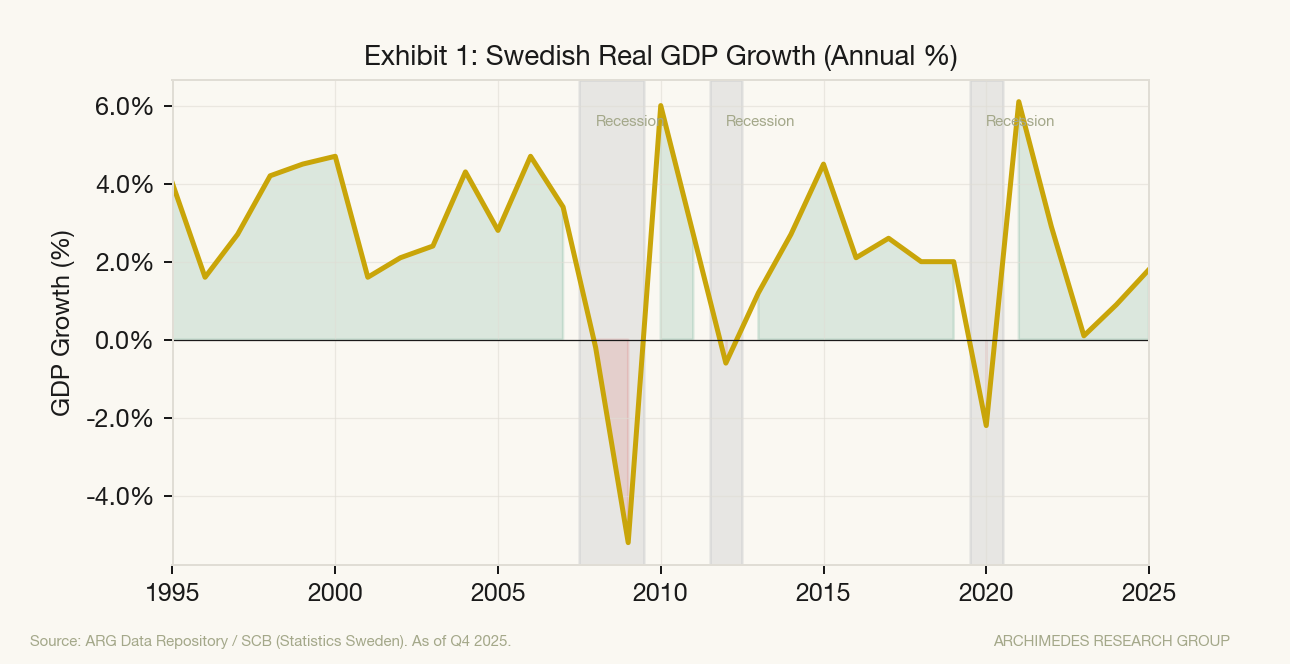
In 2008, as the Global Financial Crisis swept across Europe, Sweden's GDP contracted by more than 5% — one of the sharpest declines among advanced economies. The country had only been measuring quarterly GDP since 1993, and its modern macroeconomic toolkit was barely fifteen years old. Yet the speed and depth of the downturn posed a question that resonates well beyond Scandinavia: would the same indicators that reliably signal recessions in the United States have provided warning in Sweden?

Most business cycle research centers on the United States. That makes sense — the U.S. produces the deepest set of high-frequency economic data in the world, and the NBER's recession dating methodology has set the standard for how economists think about cyclical turning points. But anchoring exclusively to one economy creates blind spots. Variables that are powerful predictors in the U.S. may behave differently in economies with different structures, trade exposures, and institutional histories.

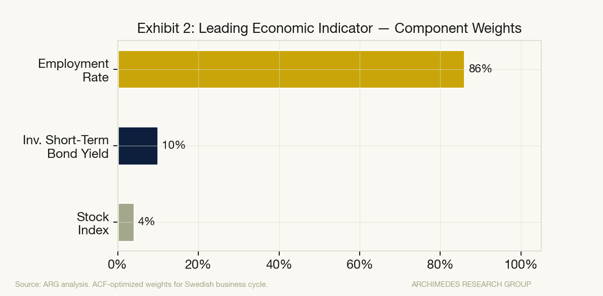
Sweden offers an instructive contrast. It is a small, open, export-driven economy where exports account for roughly 47% of GDP — compared to about 12% in the United States.

It has a highly egalitarian income distribution (Gini index of 29.25, placing it in the 83rd percentile globally) and a services-dominated GDP composition typical of advanced economies: 66% services, 21% industry, and 11% agriculture. Its population of 10.4 million and GDP of approximately $635 billion put it in a category that is economically sophisticated but structurally distinct from the large, consumption-driven U.S. economy.

Critically, Sweden's modern macroeconomic measurement infrastructure is relatively young. Quarterly GDP was not measured until 1993, following a nationwide financial crisis from 1990 to 1994 that was triggered by a housing bubble, a credit crunch, and widespread banking insolvency. That crisis served as the catalyst for developing more mature economic measurement tools — a pattern that repeats across economic history. Crises drive measurement. Since 1993, Sweden has experienced four technical recessions measured on a quarterly basis, providing a meaningful sample for testing indicator behavior across multiple cycles.

Building the Indicator Framework

The goal of this analysis was to construct both a Leading Economic Indicator (LEI) and a Coincident Economic Indicator (CEI) for the Swedish economy — not by importing assumptions from the U.S. framework, but by letting the data determine which variables lead, coincide with, or lag GDP in Sweden specifically.

The process follows a disciplined methodology. First, assemble a set of candidate variables that plausibly relate to economic activity: confidence surveys, equity markets, bond yields, construction permits, industrial production, retail sales, and employment. Second, graph each variable alongside GDP and visually assess the relationship. Third, use cross-correlation analysis — essentially measuring how strongly each variable tracks GDP at different time offsets — to statistically determine whether a given variable leads, coincides with, or lags economic output. Fourth, select the variables with the strongest leading or coincident properties. Fifth, construct composite indices by calculating monthly percentage changes in each selected variable and weighting them by their relative explanatory power.

This is the same essential methodology that underpins the Conference Board's indicators in the United States, the OECD's Composite Leading Indicators, and — in a more refined form — the indicator suite we are building at Archimedes Research Group. The framework is universal. The specific answers it produces are not.

What the Data Revealed

The cross-correlation analysis produced a clear classification of each variable's relationship to Swedish GDP — and the results were not what a U.S.-trained economist would necessarily expect. Some variables behaved as predicted. Others diverged sharply from the roles they play in American business cycle analysis.

| Variable | Classification | ACF Peak Lag | Key Observation | |----------|---|---|---| | Employment Rate | Leading | 2 quarters | GDP lags employment changes — opposite of the U.S. pattern | | Short-Term Bond Yields (3-month, inverse) | Leading | 3–4 quarters | The strongest leading signal, consistent with monetary policy transmission | | Stock Market Index | Coincident | 0 quarters | Moves in real-time with GDP; slight positive skew suggests marginal leading properties | | Retail Sales Index | Coincident | 0 quarters | Near-perfect coincident behavior | | Industrial Production | Coincident | 0 quarters | Strong positive correlation; subject to some autocorrelation as GDP component | | Building Permits | Coincident | 0 quarters | Weaker correlation due to seasonality; improved after seasonal adjustment | | Long-Term Bond Yields | Coincident | 0 quarters | Coincident despite being leading indicator in many other countries | | Economic Tendency Indicator | Lagging | 2 quarters | Lags GDP — confidence surveys reflect rather than predict conditions |

The most consequential finding was the behavior of employment. In the United States, the unemployment rate is a classic lagging indicator — it peaks well after a recession has ended and troughs well after an expansion is mature. In Sweden, employment exhibited leading properties, with GDP changes following employment changes by approximately two quarters. This likely reflects the structural characteristics of Sweden's labor market: strong union protections, active labor market policies, and an export-driven economy where hiring and hours adjustments propagate through the economy more quickly than in the U.S. services sector.

Equally notable was the behavior of long-term government bond yields. In the United States, the yield curve — particularly the 10-year minus 3-month Treasury spread — is among the most reliable recession predictors in existence. In Sweden, long-term yields behaved as a coincident indicator, moving simultaneously with GDP rather than leading it. The short end of the curve, however, did provide a genuine leading signal of three to four quarters, consistent with the transmission lag of Riksbank monetary policy.

Constructing the Composite Indicators

Based on the cross-correlation results, two composite indices were constructed.

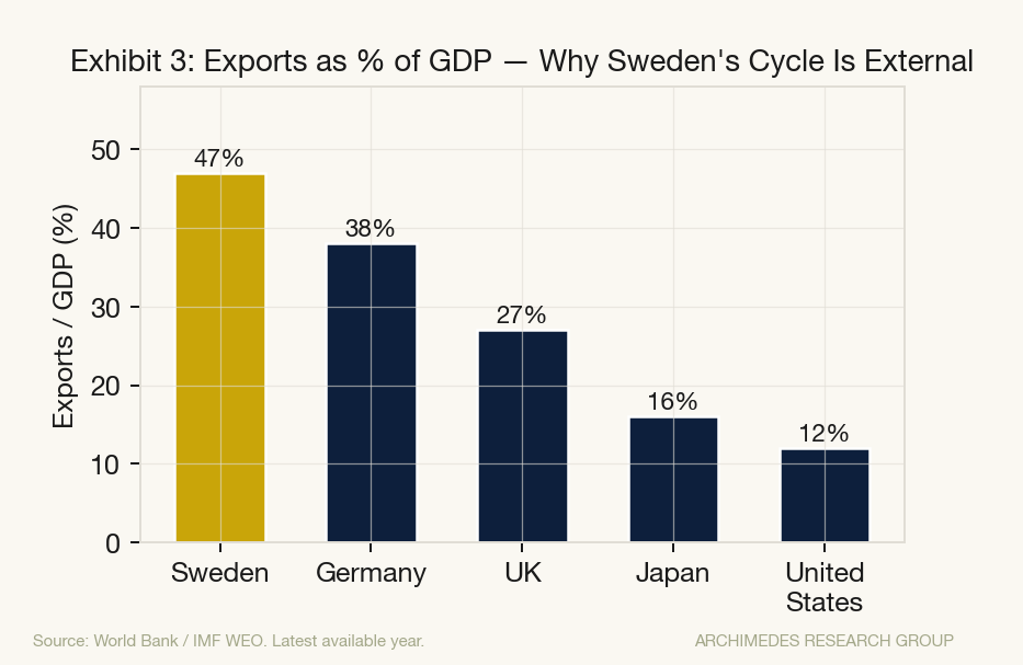
The Leading Economic Indicator combined three variables: the stock market index, the employment rate, and inverse short-term (3-month) bond yields. Each variable was standardized using inverse standard deviation weighting — a technique that ensures more volatile series do not disproportionately drive the composite signal. The employment rate received the highest weight (0.86), reflecting its low volatility and strong predictive consistency, followed by the inverse short-term yield (0.10) and the stock index (0.04).

The Coincident Economic Indicator combined four variables: building permits, the Economic Tendency Indicator, industrial production output, and retail sales. Industrial production received the dominant weight (0.52) due to its tight correlation with GDP and low relative volatility, followed by the Economic Tendency Indicator (0.40), retail sales (0.08), and building permits (0.01).

How Well Did They Work?

The CEI tracked real GDP growth with strong fidelity across the sample period. It captured the depth and duration of each of Sweden's four post-1993 recessions, including the sharp 2009 contraction during the Global Financial Crisis and the brief but severe COVID-19 downturn in early 2020. This is the expected behavior of a well-constructed coincident index — it should confirm in real time what GDP tells you quarterly.

The LEI told a more complex story. In earlier periods, it provided a clear leading signal, with turning points in the index consistently preceding turning points in GDP growth. However, in more recent years — particularly during the era of negative interest rates in Sweden from roughly 2015 to 2019 — the bond yield component introduced significant volatility into the index. When yields approach zero or turn negative, the inverse transformation amplifies small movements into outsized swings, distorting the composite signal.

Removing long-term bond yields from the LEI (which had been initially included as a candidate) reduced this fluctuation meaningfully and produced a cleaner signal. But the short-term yield component, while correctly classified as leading, still generated noise in the zero-lower-bound environment. When Sweden's Riksbank pushed its policy rate to -0.50% in 2016, the inverse transformation of yields produced readings that were more mathematical artifact than economic signal.

This is not a problem unique to Sweden — it is a structural challenge that any yield-curve-based indicator faces in an era of unconventional monetary policy. The question it raises is whether indicators built during one monetary regime remain reliable when that regime changes fundamentally.

The Broader Lesson

The Sweden case study illustrates a principle that is central to how we build indicators at Archimedes Research Group: the relationship between economic variables and the business cycle is not fixed. It varies across countries, across time periods, and across monetary policy regimes. An indicator framework that mechanically imports the U.S. playbook — treating the yield curve as a leading indicator, unemployment as lagging, and consumer confidence as coincident — will produce misleading signals in economies where those relationships do not hold.

This has direct implications for U.S. indicator construction as well. The yield curve inversion of 2022–2024 was the longest and deepest since the 1980s, and yet the widely anticipated recession did not materialize within the typical twelve-to-eighteen-month lag. One reason is that the relationship between the yield curve and real economic activity may be shifting in a post-quantitative-easing world where the term premium is distorted by central bank balance sheet policy. The same structural issue that corrupted our Swedish LEI in a negative-rate environment is present, in milder form, in the United States today.

The solution is not to abandon any single variable but to build composite indicators that are robust to these structural shifts — drawing on multiple data sources, validating against multiple cycles, and regularly re-evaluating the signal properties of each component. That is the approach we take with the ARG Recession Probability Model, the ARG Financial Conditions Index, and the broader suite of indicators we publish. The methodology is the same one applied in this Swedish analysis, adapted to the U.S. data environment and stress-tested against six recessions going back to 1980.

Business cycles are fundamentally similar across advanced economies — they share common drivers in credit conditions, confidence, trade, and monetary policy. But the specific way those drivers manifest in observable data is highly context-dependent. The only way to build indicators that actually work is to let the data tell you what leads, what follows, and what moves in real time. Assumptions are the enemy of accuracy.

Notes & Sources

Statistics Sweden (SCB). National Accounts, quarterly GDP data. Constant local currency units, seasonally adjusted. scb.se.
OECD. Sweden Economic Tendency Indicator, quarterly. data.oecd.org.
Riksbank (Sweden's central bank). Government bond yields, 3-month and long-term. riksbank.se.
Federal Reserve Bank of St. Louis (FRED). Swedish GDP (CLVMNACSCAB1GQSE), Swedish technical recession indicators. fred.stlouisfed.org.
The Conference Board. Composite Index methodology: leading, coincident, and lagging indicator construction. conference-board.org.
OECD. Composite Leading Indicators: methodology and country coverage. oecd.org/leading-indicators.

About Archimedes Research Group: Archimedes Research Group is an independent economic research and intelligence firm. We develop proprietary macroeconomic indicators, publish data-driven research, and provide advisory services to investment managers, corporate finance teams, financial institutions, and policy organizations. Our work is anchored in public data and transparent methodology.